The notebook is available here: https://github.com/starkit/starkit/tree/master/docs/examples/photometry_spectroscopy_fit.ipynb
Fitting photometry and a spectrum together
This example fits a synthetic star three ways: with its spectrum, with its SDSS colors, and with both together. The star is computed from the test grid phoenix_t4000_10000_w3000_9000_r3000.h5, which covers 3000 to 9000 Å, so the fitted values can be compared with the input ones. The fits use MultiNest, which needs the pymultinest package and the MultiNest library (see Installation and Fitting); the three fits take about half a minute in total.
[1]:
import logging
import time
import warnings

import matplotlib.pyplot as plt
import numpy as np
import pandas as pd
from astropy import units as u

from starkit import assemble_model
from starkit.fitkit.likelihoods import (Addition, PhotometryColorLikelihood,
                                        SpectralChi2Likelihood)
from starkit.fitkit.multinest import MultiNest
from starkit.fitkit.priors import UniformPrior
from starkit.fix_spectrum1d import SKSpectrum1D
from starkit.gridkit import load_grid

logging.getLogger('starkit').setLevel(logging.WARNING)
# The normalization warns about every full-rank polynomial fit (BUGS.md).
warnings.filterwarnings('ignore', message='The fit may be poorly conditioned')
# The flux unit label of the grid, erg/s/angstrom, has several slashes.
warnings.filterwarnings('ignore', message='.*contains multiple slashes')
The synthetic star
The star has \(T_\mathrm{eff}\) = 5780 K, \(\log g\) = 4.4, [M/H] = -0.3, a radial velocity of 25 km/s and an extinction \(A_V\) = 0.5 mag (\(R_V\) = 3.1).
[2]:
grid = load_grid('phoenix_t4000_10000_w3000_9000_r3000.h5',
                 wavelength_type='vacuum')
truth = {'teff': 5780., 'logg': 4.4, 'mh': -0.3, 'vrad': 25., 'a_v': 0.5}
grid.teff, grid.logg, grid.mh = truth['teff'], truth['logg'], truth['mh']
The spectrum is made as in Fitting: the model between 5000 and 5500 Å, shifted by the radial velocity, normalized to its median, with Gaussian noise for a signal-to-noise ratio of 50 per pixel. The normalization removes the continuum shape, so the spectrum carries no information on the extinction.
[3]:
wavelength, flux = assemble_model(grid, vrad=truth['vrad'])()
in_range = (wavelength > 5000) & (wavelength < 5500)
obs_wavelength = wavelength[in_range][::2]
obs_flux = np.interp(obs_wavelength, wavelength, flux)
obs_flux /= np.median(obs_flux)
obs_uncertainty = obs_flux / 50.
obs_flux += np.random.default_rng(0).normal(0., obs_uncertainty)
spectrum = SKSpectrum1D.from_array(
    wavelength=obs_wavelength * u.angstrom,
    flux=obs_flux * u.Unit('erg / (s cm2 Angstrom)'),
    uncertainty=obs_uncertainty)
print(f'{obs_wavelength.size} pixels from {obs_wavelength[0]:.1f} to '
      f'{obs_wavelength[-1]:.1f} Angstrom')
572 pixels from 5000.0 to 5499.3 Angstrom
The photometry is in the SDSS u, g, r and i filters, with curves from the SVO Filter Profile Service. SDSS z is left out: 42% of its response lies beyond the 9000 Å limit of the grid, and Photometry refuses a filter with more than 1% of its response outside the spectrum. SDSS magnitudes are on the AB system, so mag_type='ab'. The magnitudes are those of the reddened model, with Gaussian noise of 0.02 mag.
The grid holds the flux at the stellar surface, so the magnitudes are those of the stellar surface (see Grid flux units). Their differences, the colors, do not depend on the radius or the distance of the star, and the fits below use only the colors.
[4]:
sdss = ['SLOAN/SDSS.u', 'SLOAN/SDSS.g', 'SLOAN/SDSS.r', 'SLOAN/SDSS.i']
true_magnitudes = assemble_model(grid, filter_set=sdss, mag_type='ab',
                                 a_v=truth['a_v'])()
magnitude_uncertainties = np.full(len(sdss), 0.02)
observed_magnitudes = true_magnitudes + np.random.default_rng(1).normal(
    0., magnitude_uncertainties)
pd.DataFrame({'model': true_magnitudes, 'observed': observed_magnitudes,
              'uncertainty': magnitude_uncertainties},
             index=sdss).round(4)
[4]:
| model | observed | uncertainty | |
|---|---|---|---|
| SLOAN/SDSS.u | -36.1444 | -36.1375 | 0.02 |
| SLOAN/SDSS.g | -37.4879 | -37.4715 | 0.02 |
| SLOAN/SDSS.r | -38.0934 | -38.0868 | 0.02 |
| SLOAN/SDSS.i | -38.3133 | -38.3394 | 0.02 |
The likelihoods
Each likelihood is a model followed by a likelihood operation.
The spectrum:
SpectralChi2Likelihoodcompares the observed spectrum with the model, shifted by the radial velocity and normalized with a polynomial of degree 3.The colors:
PhotometryColorLikelihoodcompares the colors u - g, g - r and r - i with those of the model, reddened witha_v, using the covariance of adjacent colors, which share a magnitude.Both:
assemble_modelwith a spectrum andfilter_setsends the model spectrum both to the spectrograph operations and toPhotometry. The two likelihood operations are joined with&, andAdditionadds their logarithms. The extinction is applied to the magnitudes only.
r_v is a fixed parameter of the extinction, held at 3.1.
[5]:
spectrum_likelihood = (
    assemble_model(grid, spectrum=spectrum, vrad=0., normalize_npol=3)
    | SpectralChi2Likelihood(spectrum))
color_likelihood = (
    assemble_model(grid, filter_set=sdss, mag_type='ab', a_v=0.)
    | PhotometryColorLikelihood(observed_magnitudes, magnitude_uncertainties))
combined_likelihood = (
    assemble_model(grid, spectrum=spectrum, filter_set=sdss, mag_type='ab',
                   vrad=0., a_v=0., normalize_npol=3)
    | (SpectralChi2Likelihood(spectrum)
       & PhotometryColorLikelihood(observed_magnitudes,
                                   magnitude_uncertainties))
    | Addition())
likelihoods = {'spectrum': spectrum_likelihood, 'colors': color_likelihood,
               'combined': combined_likelihood}


def free_parameters(likelihood):
    return [name for name in likelihood.param_names
            if not getattr(likelihood, name).fixed]


for name, likelihood in likelihoods.items():
    print(f'{name:9s}', free_parameters(likelihood))
spectrum  ['teff_0', 'logg_0', 'mh_0', 'vrad_1']
colors    ['teff_0', 'logg_0', 'mh_0', 'a_v_1']
combined  ['teff_0', 'logg_0', 'mh_0', 'vrad_1', 'a_v_5']
The fits
MultiNest needs a prior for each free parameter, in the order of free_parameters. The priors are uniform: over the grid for \(T_\mathrm{eff}\), \(\log g\) and [M/H], from -100 to 100 km/s for the radial velocity, and from 0 to 3 mag for \(A_V\). With the seed, running the notebook from the top reproduces the outputs below; a fit run on its own, or after other fits, gives slightly different numbers.
[6]:
grid_priors = dict(zip(grid.param_names, grid.get_grid_uniform_priors()))
other_priors = {'vrad': UniformPrior(-100., 100.), 'a_v': UniformPrior(0., 3.)}


def base_name(parameter):
    # teff_0 -> teff, a_v_4 -> a_v
    return parameter[:parameter.rfind('_')]


def priors_for(likelihood):
    priors = []
    for parameter in free_parameters(likelihood):
        name = base_name(parameter)
        priors.append(grid_priors[name] if name in grid_priors
                      else other_priors[name])
    return priors


results = {}
for name, likelihood in likelihoods.items():
    start = time.time()
    fitter = MultiNest(likelihood, priors_for(likelihood))
    results[name] = fitter.run(seed=1)
    print(f'{name:9s} {time.time() - start:5.0f} s')
 MultiNest Warning: no resume file found, starting from scratch
 *****************************************************
 MultiNest v3.10
 Copyright Farhan Feroz & Mike Hobson
 Release Jul 2015

 no. of live points =  400
 dimensionality =    4
 *****************************************************
 ln(ev)=  -297.26116969113650      +/-  0.15865374635665447
 Total Likelihood Evaluations:         9928
 Sampling finished. Exiting MultiNest
spectrum      2 s
 MultiNest Warning: no resume file found, starting from scratch
 *****************************************************
 MultiNest v3.10
 Copyright Farhan Feroz & Mike Hobson
 Release Jul 2015

 no. of live points =  400
 dimensionality =    4
 *****************************************************
 ln(ev)=  -5.7318868961215967      +/-  0.10885266015592368
 Total Likelihood Evaluations:         5120
 Sampling finished. Exiting MultiNest
colors        8 s
 MultiNest Warning: no resume file found, starting from scratch
 *****************************************************
 MultiNest v3.10
 Copyright Farhan Feroz & Mike Hobson
 Release Jul 2015

 no. of live points =  400
 dimensionality =    5
 *****************************************************
 ln(ev)=  -301.96844395294499      +/-  0.18257664754136277
 Total Likelihood Evaluations:        13027
 Sampling finished. Exiting MultiNest
combined     21 s
Results
The table gives the median of each posterior and, after it, the distances from the median to the upper and lower limits of the central 68% of the posterior.
[7]:
labels = {'teff': 'Teff (K)', 'logg': 'log g', 'mh': '[M/H]',
          'vrad': 'v_rad (km/s)', 'a_v': 'A_V (mag)'}
digits = {'teff': 0, 'logg': 2, 'mh': 3, 'vrad': 2, 'a_v': 3}


def posterior_column(result, name):
    columns = [c for c in result.parameter_names if base_name(c) == name]
    return columns[0] if columns else None


rows = {}
for name, label in labels.items():
    row = {'input': f'{truth[name]:.{digits[name]}f}'}
    for fit, result in results.items():
        column = posterior_column(result, name)
        if column is None:
            row[fit] = ''
            continue
        median = result.median[column]
        lower, upper = result.calculate_sigmas(1)[column]
        row[fit] = (f'{median:.{digits[name]}f} '
                    f'+{upper - median:.{digits[name]}f} '
                    f'-{median - lower:.{digits[name]}f}')
    rows[label] = row
pd.DataFrame(rows).T
[7]:
| input | spectrum | colors | combined | |
|---|---|---|---|---|
| Teff (K) | 5780 | 5718 +70 -75 | 6081 +608 -539 | 5725 +67 -70 |
| log g | 4.40 | 4.29 +0.15 -0.13 | 4.26 +0.52 -0.75 | 4.32 +0.14 -0.13 |
| [M/H] | -0.300 | -0.313 +0.055 -0.059 | -0.583 +0.289 -0.279 | -0.321 +0.052 -0.054 |
| v_rad (km/s) | 25.00 | 25.19 +2.25 -2.23 | 25.28 +2.26 -2.33 | |
| A_V (mag) | 0.500 | 0.814 +0.345 -0.363 | 0.489 +0.058 -0.059 |
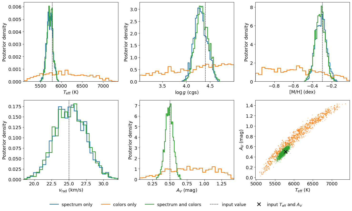
The spectrum alone gives \(T_\mathrm{eff}\) = 5718 +70 -75 K, \(\log g\) = 4.29 +0.15 -0.13, [M/H] = -0.313 +0.055 -0.059 and a radial velocity of 25.19 +2.25 -2.23 km/s; the input values lie within these 68% intervals. It gives no information on the extinction, because it is normalized.
The colors alone give \(T_\mathrm{eff}\) = 6081 +608 -539 K and \(A_V\) = 0.814 +0.345 -0.363 mag, and leave \(\log g\) and [M/H] nearly unconstrained: their posteriors spread over most of the grid. \(T_\mathrm{eff}\) and \(A_V\) are correlated (lower right panel of the posterior figure below), because a hotter star behind more extinction has nearly the same colors.
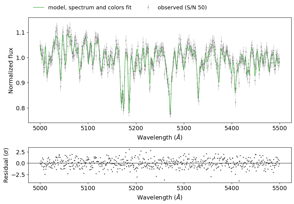
Fitting both gives \(A_V\) = 0.489 +0.058 -0.059 mag, a 68% interval of 0.12 mag against 0.71 mag from the colors alone, while \(T_\mathrm{eff}\) = 5725 +67 -70 K, \(\log g\) = 4.32 +0.14 -0.13 and [M/H] = -0.321 +0.052 -0.054 are close to the spectrum-only values. The input values of all five parameters lie within the 68% intervals. MultiNest made 9928, 5120 and 13027 likelihood evaluations for the spectrum, colors and combined fits.
The extinction law is the same in the synthetic data and in the fits (CCM89, \(R_V\) = 3.1). With observed data, a different law biases \(A_V\) and, through the colors, \(T_\mathrm{eff}\).
[8]:
FONT_KW = {'legend.fontsize': 13, 'font.size': 14, 'axes.titlesize': 15,
           'axes.labelsize': 14, 'xtick.labelsize': 14, 'ytick.labelsize': 14,
           'figure.titlesize': 16}
plt.rcParams.update(FONT_KW)
FIT_STYLE = {'spectrum': dict(color='tab:blue', label='spectrum only'),
             'colors': dict(color='tab:orange', label='colors only'),
             'combined': dict(color='tab:green', label='spectrum and colors')}


def model_at_median(fit, **keywords):
    """assemble_model(grid, **keywords) with the parameters at the medians
    of a fit; parameters the fit does not have keep the values in keywords."""
    model = assemble_model(grid, **keywords)
    median = results[fit].median
    for parameter in model.param_names:
        name = base_name(parameter)
        column = posterior_column(results[fit], name)
        if column is not None:
            setattr(model, parameter, median[column])
    return model
The observed spectrum and the model at the medians of the combined fit:
[9]:
best = model_at_median('combined', spectrum=spectrum, filter_set=sdss,
                       mag_type='ab', vrad=0., a_v=0., normalize_npol=3)
model_wavelength, model_flux, model_magnitudes = best()

fig, (ax, ax_residual) = plt.subplots(
    2, 1, figsize=(10, 7), sharex=True, height_ratios=[3, 1])
ax.errorbar(obs_wavelength, obs_flux, obs_uncertainty, fmt='.', color='0.5',
            ms=3, lw=0.5, label='observed (S/N 50)')
ax.plot(model_wavelength, model_flux, color='tab:green', lw=1,
        label='model, spectrum and colors fit')
ax.set_ylabel('Normalized flux')
ax.legend(loc='lower left', bbox_to_anchor=(0, 1.02), ncol=2, frameon=False)
ax_residual.plot(obs_wavelength, (obs_flux - model_flux) / obs_uncertainty,
                 '.', color='0.3', ms=3)
ax_residual.axhline(0, color='black', lw=0.8)
ax_residual.set_xlabel(r'Wavelength ($\AA$)')
ax_residual.set_ylabel(r'Residual ($\sigma$)')
ax.tick_params(labelbottom=True)
ax.set_xlabel(r'Wavelength ($\AA$)')
fig.tight_layout()
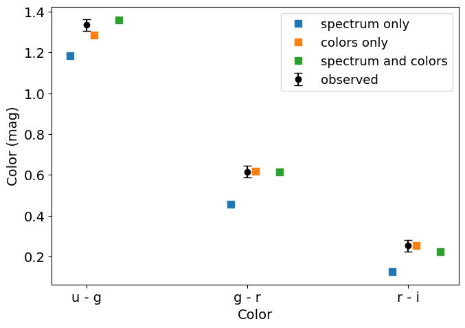
The observed colors and those of the model at the medians of each fit. The spectrum-only fit has no extinction, so its colors are those of the unreddened model.
[10]:
def colors(magnitudes):
    return np.asarray(magnitudes)[:-1] - np.asarray(magnitudes)[1:]


color_names = ['u - g', 'g - r', 'r - i']
x = np.arange(len(color_names))
fig, ax = plt.subplots(figsize=(7, 5))
ax.errorbar(x, colors(observed_magnitudes),
            np.sqrt(2) * magnitude_uncertainties[1:], fmt='o', color='black',
            capsize=4, label='observed')
for offset, fit in zip([-0.15, 0.0, 0.15], results):
    model = model_at_median(fit, filter_set=sdss, mag_type='ab', a_v=0.)
    ax.plot(x + offset + 0.05, colors(model()), 's', ms=7,
            **FIT_STYLE[fit])
ax.set_xticks(x)
ax.set_xticklabels(color_names)
ax.set_xlabel('Color')
ax.set_ylabel('Color (mag)')
ax.legend()
fig.tight_layout()
The posterior distributions of the three fits, with the input values as vertical lines, and 2000 samples of \(T_\mathrm{eff}\) and \(A_V\) drawn from the posteriors of the colors-only and combined fits:
[11]:
axis_labels = {'teff': r'$T_\mathrm{eff}$ (K)', 'logg': r'$\log g$ (cgs)',
               'mh': '[M/H] (dex)', 'vrad': r'$v_\mathrm{rad}$ (km/s)',
               'a_v': r'$A_V$ (mag)'}
def weighted_quantiles(values, weights, quantiles):
    order = np.argsort(values)
    cumulative = np.cumsum(np.asarray(weights)[order])
    return np.interp(quantiles, cumulative / cumulative[-1],
                     np.asarray(values)[order])


fig, axes = plt.subplots(2, 3, figsize=(15, 9))
for ax, name in zip(axes.flat, labels):
    limits = []
    for fit, result in results.items():
        column = posterior_column(result, name)
        if column is not None:
            data = result.posterior_data
            limits.extend(weighted_quantiles(data[column], data['weights'],
                                             [0.001, 0.999]))
    ax.set_xlim(min(limits), max(limits))
    for fit, result in results.items():
        column = posterior_column(result, name)
        if column is None:
            continue
        data = result.posterior_data
        low, high = weighted_quantiles(data[column], data['weights'],
                                       [0.001, 0.999])
        ax.hist(data[column], bins=np.linspace(low, high, 31),
                weights=data['weights'], density=True, histtype='step', lw=2,
                color=FIT_STYLE[fit]['color'])
    ax.axvline(truth[name], color='black', ls='--', lw=1)
    ax.set_xlabel(axis_labels[name])
    ax.set_ylabel('Posterior density')
ax = axes.flat[5]
rng = np.random.default_rng(2)
for fit in ['colors', 'combined']:
    # 2000 samples drawn with the posterior weights
    data = results[fit].posterior_data
    rows = rng.choice(len(data), size=2000,
                      p=data['weights'] / data['weights'].sum())
    ax.scatter(data[posterior_column(results[fit], 'teff')].iloc[rows],
               data[posterior_column(results[fit], 'a_v')].iloc[rows], s=3,
               alpha=0.3, color=FIT_STYLE[fit]['color'])
ax.plot(truth['teff'], truth['a_v'], 'x', color='black', ms=10, mew=2)
ax.set_xlabel(axis_labels['teff'])
ax.set_ylabel(axis_labels['a_v'])
handles = [plt.Line2D([], [], color=style['color'], lw=2, label=style['label'])
           for style in FIT_STYLE.values()]
handles.append(plt.Line2D([], [], color='black', ls='--', lw=1,
                          label='input value'))
handles.append(plt.Line2D([], [], color='black', marker='x', ls='', ms=10,
                          mew=2, label=r'input $T_\mathrm{eff}$ and $A_V$'))
fig.legend(handles=handles, loc='lower center', ncol=5, frameon=False)
fig.tight_layout(rect=[0, 0.06, 1, 1])