The notebook is available here: https://github.com/starkit/starkit/tree/master/docs/examples/solar_spectrum_fit.ipynb
Fitting the spectrum of the Sun
This example fits an observed spectrum with a grid of model spectra and compares the fitted parameters with the known values for the Sun. The spectrum is the solar irradiance atlas of Kurucz (2005; Kurucz 2006, arXiv:astro-ph/0605029), which is included with StarKit. The grid is the test grid phoenix_t4000_10000_w3000_9000_r3000.h5 in this directory.
The fit uses MultiNest, which needs the pymultinest package and the MultiNest library (see Installation), and takes about a minute. The figures need matplotlib and corner (pip install matplotlib corner).
[1]:
import logging
import time
import warnings
from importlib.resources import files

import corner
import matplotlib.pyplot as plt
import numpy as np
import pandas as pd
from astropy.table import Table

from starkit import assemble_model
from starkit.fitkit.likelihoods import SpectralChi2Likelihood
from starkit.fitkit.multinest import MultiNest
from starkit.fitkit.priors import UniformPrior
from starkit.fix_spectrum1d import SKSpectrum1D
from starkit.gridkit import load_grid

logging.getLogger('starkit').setLevel(logging.WARNING)
# The normalization warns about every full-rank polynomial fit (BUGS.md).
warnings.filterwarnings('ignore', message='The fit may be poorly conditioned')
# The flux unit label of the grid, erg/s/angstrom, has several slashes.
warnings.filterwarnings('ignore', message='.*contains multiple slashes')
The solar spectrum
The atlas is made from Fourier transform spectra of the Sun taken at Kitt Peak, with the telluric lines divided out, and calibrated to the solar irradiance of Thuillier et al. (2004). Its wavelengths are vacuum wavelengths in the rest frame of the Sun and include the gravitational redshift of the solar spectrum, 0.64 km/s. The file sun_kurucz2005_r1500.fits in the starkit/data directory holds the irradiance at Earth in W m\(^{-2}\) nm\(^{-1}\) from 3010 to 9000 Å, smoothed to
a resolving power \(R = \lambda / \Delta\lambda = 1500\) (\(\Delta\lambda\) is the FWHM of a Gaussian line profile) and sampled on the wavelengths of the grid. The name of the grid says \(R = 3000\), but its spectra have \(R = 1500\) (see BUGS.md), and an observed spectrum must not have a higher resolving power than the grid it is fitted with. The script make_solar_spectrum.py in this directory makes the file from the atlas.
[2]:
sun = Table.read(files('starkit') / 'data' / 'sun_kurucz2005_r1500.fits')
print(sun.meta['REFERENC'])
sun[:3]
Kurucz, R. L. 2006, arXiv:astro-ph/0605029
[2]:
| WAVELENGTH | FLUX |
|---|---|
| Angstrom | W / (nm m2) |
| float64 | float64 |
| 3010.0166852005304 | 0.45825735035046533 |
| 3010.267530376032 | 0.48909447220077834 |
| 3010.5183964561693 | 0.5240649017823544 |
The fit uses 3800 to 8950 Å. The upper limit keeps the model, shifted by up to 50 km/s, inside the 9000 Å end of the grid.
The atlas gives no uncertainty for each flux point, so this example assumes a signal-to-noise ratio of 100 per point: the uncertainty is 1% of the flux. For your own spectrum, give the measured uncertainty of each flux point instead. The widths of the posteriors below scale with the uncertainties.
[3]:
in_range = (sun['WAVELENGTH'] > 3800) & (sun['WAVELENGTH'] < 8950)
wavelength = sun['WAVELENGTH'][in_range].quantity
flux = sun['FLUX'][in_range].quantity
uncertainty = flux.value / 100.  # assumed signal-to-noise ratio of 100
spectrum = SKSpectrum1D.from_array(wavelength=wavelength, flux=flux,
                                   uncertainty=uncertainty)
print(f'{len(wavelength)} points from {wavelength[0]:.1f} to '
      f'{wavelength[-1]:.1f}')
10280 points from 3800.1 Angstrom to 8949.6 Angstrom
The model and the likelihood
assemble_model builds the model for the observed spectrum: it interpolates the grid at \(T_\mathrm{eff}\), \(\log g\) and [M/H], shifts the spectrum by the radial velocity vrad (km/s), interpolates it onto the observed wavelengths, and multiplies it by the polynomial in wavelength of degree 10 (normalize_npol=10) that best matches the observed spectrum. The polynomial takes up the flux scale, since the grid holds the flux at the stellar surface and the atlas the irradiance at
Earth, and any error in the flux calibration. It also takes up most of the slope of the continuum, so the fit uses mainly the absorption lines. SpectralChi2Likelihood turns the model into the log-likelihood \(-\chi^2/2\).
[4]:
grid = load_grid('phoenix_t4000_10000_w3000_9000_r3000.h5',
                 wavelength_type='vacuum')
model = assemble_model(grid, spectrum=spectrum, vrad=0., normalize_npol=10)
likelihood = model | SpectralChi2Likelihood(spectrum)
free_parameters = [name for name in likelihood.param_names
                   if not getattr(likelihood, name).fixed]
free_parameters
[4]:
['teff_0', 'logg_0', 'mh_0', 'vrad_1']
The fit
MultiNest needs a prior for each free parameter, in the order of free_parameters. The priors are uniform: over the grid for \(T_\mathrm{eff}\) (4000 to 10000 K), \(\log g\) (3.0 to 5.0) and [M/H] (-1.0 to 0.0), and from -50 to 50 km/s for the radial velocity. The solar [M/H] of 0.0 is at the upper edge of the grid. With the seed, running the notebook from the top reproduces the outputs below, apart from the run time.
[5]:
priors = grid.get_grid_uniform_priors() + [UniformPrior(-50., 50.)]
fitter = MultiNest(likelihood, priors)
start = time.time()
result = fitter.run(seed=1)
print(f'{time.time() - start:.0f} s')
 MultiNest Warning: no resume file found, starting from scratch
 *****************************************************
 MultiNest v3.10
 Copyright Farhan Feroz & Mike Hobson
 Release Jul 2015

 no. of live points =  400
 dimensionality =    4
 *****************************************************
 ln(ev)=  -22938.602688210340      +/-  0.23927456411051992
 Total Likelihood Evaluations:        19290
 Sampling finished. Exiting MultiNest
55 s
Results
The table gives the median of each posterior, the distances from the median to the limits of the central 68% of the posterior, and the solar values: \(T_\mathrm{eff}\) = 5772 K and \(\log g\) = 4.44 from the nominal solar values of IAU 2015 Resolution B3 (Prša et al. 2016, AJ 152, 41), [M/H] = 0.0, and a radial velocity of 0.64 km/s, the gravitational redshift that the atlas includes.
[6]:
solar = {'teff_0': 5772., 'logg_0': 4.44, 'mh_0': 0.0, 'vrad_1': 0.64}
labels = {'teff_0': 'Teff (K)', 'logg_0': 'log g', 'mh_0': '[M/H]',
          'vrad_1': 'v_rad (km/s)'}
digits = {'teff_0': 0, 'logg_0': 3, 'mh_0': 3, 'vrad_1': 2}
limits = result.calculate_sigmas(1)
rows = {}
for name, label in labels.items():
    median = result.median[name]
    lower, upper = limits[name]
    n = digits[name]
    rows[label] = {'median': f'{median:.{n}f}',
                   '68% interval': f'+{upper - median:.{n}f} -{median - lower:.{n}f}',
                   'Sun': f'{solar[name]:.{n}f}',
                   'median - Sun': f'{median - solar[name]:+.{n}f}'}
pd.DataFrame(rows).T
[6]:
| median | 68% interval | Sun | median - Sun | |
|---|---|---|---|---|
| Teff (K) | 5805 | +1 -1 | 5772 | +33 |
| log g | 4.343 | +0.003 -0.003 | 4.440 | -0.097 |
| [M/H] | -0.129 | +0.003 -0.003 | 0.000 | -0.129 |
| v_rad (km/s) | -0.78 | +0.21 -0.19 | 0.64 | -1.42 |
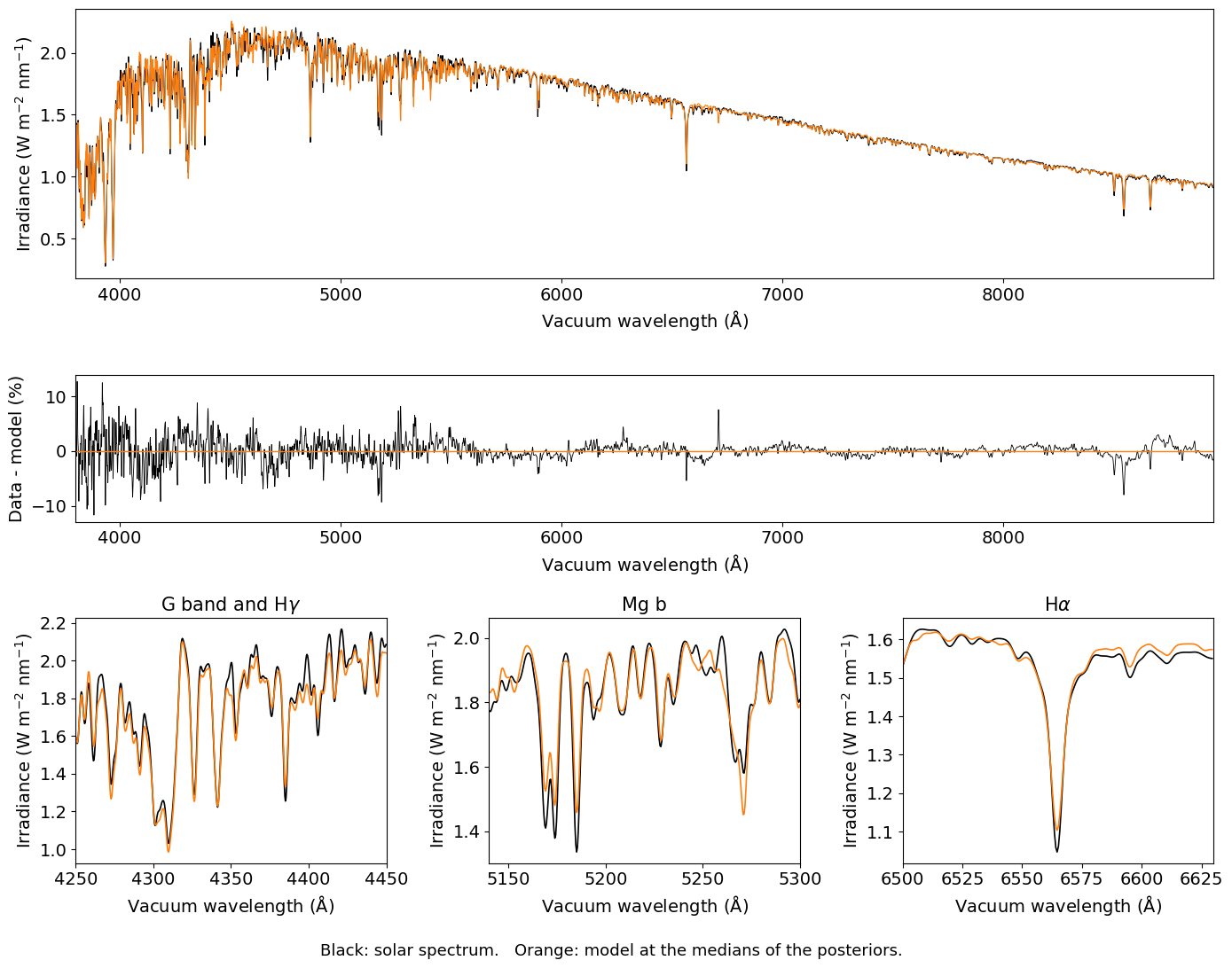
The model at the medians of the posteriors, and its \(\chi^2\) per flux point:
[7]:
for name in free_parameters:
    setattr(model, name, result.median[name])
model_wavelength, model_flux = model()
observed_flux = flux.value
chi2 = np.sum(((observed_flux - model_flux) / uncertainty)**2)
print(f'chi2 per flux point: {chi2 / observed_flux.size:.2f}')
difference = 100 * (observed_flux - model_flux) / observed_flux
blue = wavelength.value < 4500
for part, name in [(blue, 'below'), (~blue, 'above')]:
    rms = np.sqrt(np.mean(difference[part]**2))
    print(f'rms difference {name} 4500 Angstrom: {rms:.2f}%')
chi2 per flux point: 4.46
rms difference below 4500 Angstrom: 3.66%
rms difference above 4500 Angstrom: 1.50%
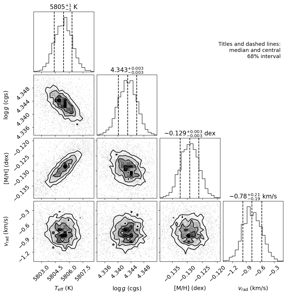
The fitted \(T_\mathrm{eff}\) is 33 K above the solar value, \(\log g\) is 0.097 lower and [M/H] is 0.129 dex lower. The radial velocity of -0.78 km/s is 1.42 km/s below the gravitational redshift, a difference small compared with the 25 km/s spacing of the grid wavelengths.
These differences are many times the 68% intervals of the posteriors (1 K in \(T_\mathrm{eff}\), 0.003 in \(\log g\) and in [M/H], 0.2 km/s in the radial velocity). The posteriors assume that the model matches the spectrum to within the assumed uncertainty of 1%. The fit is dominated by systematic errors in the model rather than statistical errors. The model and the spectrum differ by 3.66% rms below 4500 Å and 1.50% above. The middle panel of the figure below shows the differences; they are largest below 4500 Å, in the Mg b lines at 5165 to 5185 Å, in the Ca II lines near 8500 Å, and at 6710 Å, where the model has an absorption line that is nearly absent from the atlas. The posterior widths therefore understate the errors of the fitted parameters. For this grid at \(R = 1500\), the differences from the solar values are a better indication of the error of a fit to a star like the Sun.
An additional systematic error likely is needed to be added to the statistical errors.
The observed spectrum with the model, their difference, and three regions in detail:
[8]:
FONT_KW = {'legend.fontsize': 13, 'font.size': 14, 'axes.titlesize': 15,
           'axes.labelsize': 14, 'xtick.labelsize': 14, 'ytick.labelsize': 14,
           'figure.titlesize': 16}
plt.rcParams.update(FONT_KW)
w = wavelength.value
flux_label = r'Irradiance (W m$^{-2}$ nm$^{-1}$)'
wavelength_label = r'Vacuum wavelength ($\mathrm{\AA}$)'

fig = plt.figure(figsize=(14, 11))
grid_spec = fig.add_gridspec(3, 3, height_ratios=[2.2, 1.2, 2])
ax = fig.add_subplot(grid_spec[0, :])
ax.plot(w, observed_flux, color='black', lw=0.8)
ax.plot(w, model_flux, color='tab:orange', lw=0.8)
ax.set_xlim(w[0], w[-1])
ax.set_xlabel(wavelength_label)
ax.set_ylabel(flux_label)

ax = fig.add_subplot(grid_spec[1, :])
ax.plot(w, 100 * (observed_flux - model_flux) / observed_flux, color='black',
        lw=0.6)
ax.axhline(0, color='tab:orange', lw=1)
ax.set_xlim(w[0], w[-1])
ax.set_xlabel(wavelength_label)
ax.set_ylabel('Data - model (%)')

regions = [(4250, 4450, r'G band and H$\gamma$'), (5140, 5300, 'Mg b'),
           (6500, 6630, r'H$\alpha$')]
for i, (low, high, title) in enumerate(regions):
    ax = fig.add_subplot(grid_spec[2, i])
    shown = (w > low) & (w < high)
    ax.plot(w[shown], observed_flux[shown], color='black', lw=1.2)
    ax.plot(w[shown], model_flux[shown], color='tab:orange', lw=1.2)
    ax.set_xlim(low, high)
    ax.set_title(title)
    ax.set_xlabel(wavelength_label)
    ax.set_ylabel(flux_label)

fig.text(0.5, 0.01, 'Black: solar spectrum.   Orange: model at the medians '
         'of the posteriors.', ha='center', fontsize=13)
fig.tight_layout(rect=(0, 0.03, 1, 1))
The posteriors in a corner plot. The solar values lie outside the plotted range of every parameter (see the table above), so they are not drawn.
[9]:
axis_labels = [r'$T_\mathrm{eff}$ (K)', r'$\log g$ (cgs)', '[M/H] (dex)',
               r'$v_\mathrm{rad}$ (km/s)']
title_units = [' K', '', ' dex', ' km/s']
# Median and central 68.3% interval, as in the table above.
interval = [0.1587, 0.5, 0.8413]
fig = plt.figure(figsize=(10, 10))
corner.corner(result.posterior_data[free_parameters].to_numpy(),
              weights=result.posterior_data['weights'].to_numpy(),
              labels=axis_labels, range=[0.999] * len(free_parameters),
              quantiles=interval, label_kwargs={'fontsize': 14},
              labelpad=0.1, fig=fig)
axes = np.array(fig.axes).reshape(len(free_parameters), len(free_parameters))
for i, name in enumerate(free_parameters):
    median = result.median[name]
    lower, upper = limits[name]
    n = digits[name]
    axes[i, i].set_title(
        f'${median:.{n}f}^{{+{upper - median:.{n}f}}}'
        f'_{{-{median - lower:.{n}f}}}${title_units[i]}')
fig.text(0.95, 0.8, 'Titles and dashed lines:\nmedian and central\n68% interval',
         ha='right', fontsize=13);